Introduction
Line plots
Multiple histograms
Other plot types
Instruction
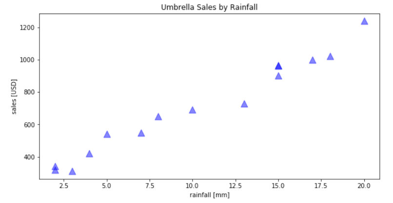
Good job. Naturally, matplotlib offers numerous other types of plots. Scatter plots are a frequent choice for many analysts. Creating them with matplotlib is very similar to creating histograms or line plots, so we won't explain everything from scratch here. Instead, take a look at the example below:
umbrellas = pd.read_csv('umbrellas.csv')
scatter_figure = plt.figure(figsize=(10, 5))
scatter_subplot = plt.subplot(111)
scatter_subplot.set_title('Umbrella Sales by Rainfall')
scatter_subplot.set_xlabel('rainfall [mm]')
scatter_subplot.set_ylabel('sales [USD]')

plt.scatter(umbrellas['rainfall'], umbrellas['sales'], c='blue', alpha=0.5, s=120, marker='^')
Take a look at the last line above. Our plt.scatter takes the following two obligatory arguments:
umbrellas['rainfall']– x-axis data,umbrellas['sales']– y-axis data.
We also added some optional arguments:
c='blue'means our points will be of colored blue,alpha=0.5means our points will be 50% transparent,s=120defines the size of our points,marker='^'means that each point will be shown as a triangle.
Exercise
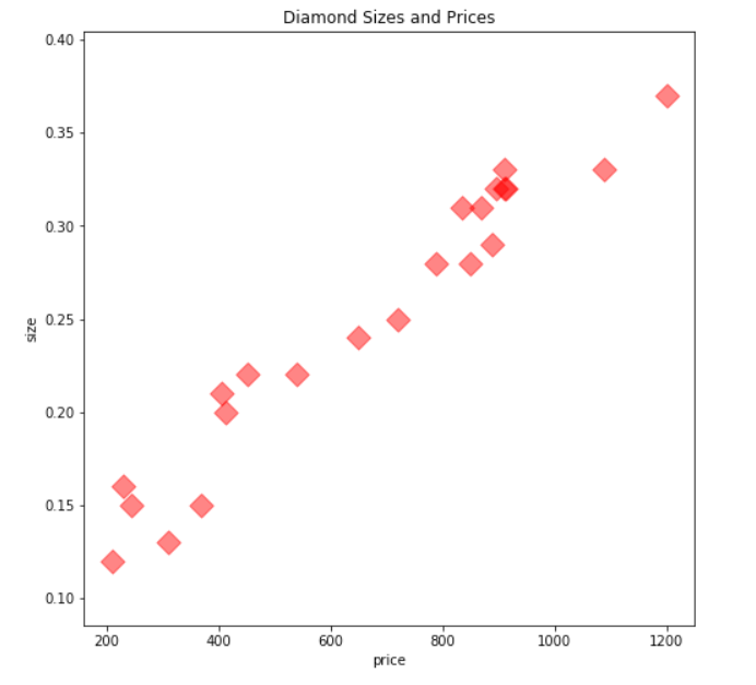
It's time for you to create your own scatter plot! Use diamond_prices.csv, which contains data about diamond sizes and their prices, and draw the following plot:
Hints:
- Use
figsize=5x5. - For plot points, use a "red" color with 50% transparency, a size of "100" and a marker "D".
- Use the
plt.subplot(111).
Stuck? Here's a hint!
Once you import the csv file, and create the subplot and the axes, you can draw the scatter plot with:
plt.scatter(diamonds['price'], diamonds['size'], c='r', alpha=0.5, s=100, marker='D')