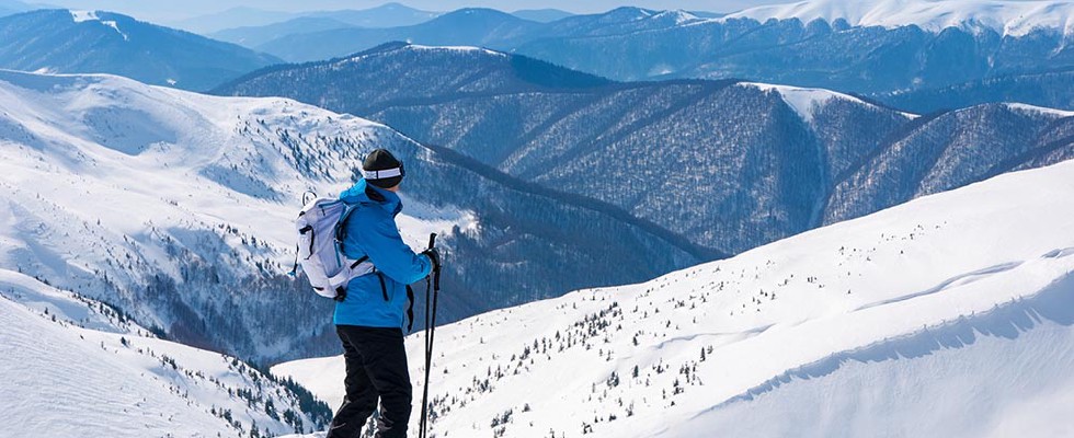
Planning a Ski Trip with R Analysis

Each year, I try to arrange some kind of birthday surprise that’ll exceed my husband’s expectations. This year, I’ve got an excellent idea—I’m going to organize a ski trip for us and a few friends with the help of R and the apply family of functions!
Overview
My husband’s loved snowboarding ever since he learned it in college, and he’s always wanted to find some time to visit our local mountains in the winter. So when January came around this year, I called up my friends and arranged a surprise—skiing in the mountains, here we come!
But we didn’t want to lose much time on travel, so we narrowed down our two main locations to Austria and Slovenia. I picked some popular skiing resorts and searched for nearby accommodations, and I saved all this info in a CSV file. Now, it’s time to decide when, where, and for what price we’ll be staying.
And for that, I’ll turn to R. Let’s get started!
Loading a CSV File in R
R can read data and create a data frame from many different sources: Excel, txt, HTML, CSV, MySQL, Oracle… The list goes on.
Simply put, a data frame is a table with rows and columns. We can load my stored trip data (ski_accommodation.csv) into an R data frame with the read.csv function:
ski_acomodation <- read.csv("ski_accomodation.csv", sep=’;’, stringsAsFactors = FALSE, dec =’,’)
After executing this code, we get a ski_acomodation data frame that contains information about various accommodations in Austria and Slovenia.
Let's use the head function to check what this table looks like. head returns the first five rows of the specified R data frame. If you try to execute following command:
head(ski_acomodation)
You’ll get this result:
| COUNTRY | DESTINATION | COST_TYPE | ACCOMODATION_NAME | COST_SUBTYPE | DATE | PRICE | RATING | DISTANCE_FROM _SKI_RESORT |
|---|---|---|---|---|---|---|---|---|
| SLOVENIA | KRVAVEC | ACCOMODATION | STAL STUDIO | STUDIO | 03.01.2019 | 702 | 9.6 | 5.2 |
| SLOVENIA | KRVAVEC | ACCOMODATION | STAL STUDIO | STUDIO | 04.01.2019 | 850 | 9.6 | 5.2 |
| SLOVENIA | KRVAVEC | ACCOMODATION | STAL STUDIO | STUDIO | 05.01.2019 | 702 | 9.6 | 5.2 |
| SLOVENIA | KRVAVEC | ACCOMODATION | PALIN APARTMENTS | HOUSE | 03.01.2019 | 1020 | 8.7 | 3.2 |
| SLOVENIA | KRVAVEC | ACCOMODATION | PALIN APARTMENTS | HOUSE | 04.01.2019 | 990 | 8.7 | 3.2 |
The table contains information about various accommodations and the associated cost of staying there for five people. Each accommodation has three rows, one for each of the days from January 3rd to January 5th. For each accommodation, we also store its rating and distance from the nearest ski resort. Besides accommodation costs, there are also travel costs (like fuel) in this table that we need to consider for reaching each accommodation.
We can easily display the two different cost types (accommodation and travel) with the following command:
unique(ski_acomodations$COST_TYPE)
Here, unique simply takes a vectorized data type (in this case, a column) and returns only unique values. In this case, it returns all unique values from the COST_TYPE column.
For now, lets eliminate travel costs from our data frame. We’re not going to analyze them just yet:
ski_acomodation_1 <- ski_acomodation[!ski_acomodation$COST_TYPE==”TRAVEL”,]
Now it’s time to pick a country to visit: Austria or Slovenia? It would be nice to find a place that is priced reasonably, has an okay rating, and is located near a ski resort.
Below is a graph depicting the prices for Austria and Slovenia:
It’s obvious from the graph that Slovenia has more acceptable prices. This cool graph was made in R with the help of plot_ly:
plot_ly(data = ski_acomodation, x = ~Price, y = ~Rating,color=~COUNTRY,colors = c(“red”,”blue”),
text=paste(‘Cost type: ‘, ski_acomodation$COST_TYPE,’,’, ‘Destination:’,ski_acomodation$DESTINATION)) %>% layout(title=”Price vs Rating”)
This is a visual approach. We can also prove that Slovenia is cheaper with some simple statistics—we can calculate the average price per night (in HRK) at the country level using this line of code:
sapply(split(ski_acomodation_1$PRICE,ski_acomodation_1$COUNTRY),mean)
R returns two figures: one for Austria, and one for Slovenia:
AUSTRIA 		SLOVENIA
5143.519 		1296.852
As you can see, Slovenia is much, much cheaper than Austria. Here, we used the sapply function. This is part of a broader family of related functions that we’ll now explore in more detail.
The apply Family of Functions
Although R has looping constructs like the for loop that are present in other languages, these aren’t commonly used. Instead of manually looping over data structures and performing repetitive tasks, we often use R apply set of functions to make our job easier.
In data science, it’s a common task to group or slice your data according to a specific key and then call a certain function on each of those slices. To that end, we can use apply/sapply in combination with another function named split.
The split Function
As you may have guessed, split divides R data frame into several slices using a specific key. It then returns a list where each element of represents one slice of that data frame. Consider this code:
split(ski_acomodations$PRICE, ski_acomodations$COUNTRY)
R returns the following list:
$AUSTRIA
[1] 2484 2210 2494 4056 4105 4200 1848 1848 1848 2395 2230 2230 5581 5481 5481 4017 4017 4017 7310 7310 7100 14569 14569
[24] 14569 4302 4302 4302

$SLOVENIA
[1] 702 850 702 1020 990 970 620 650 620 1035 1035 1035 2250 2250 2250 1271 1000 1101 1474 1200 1200 2400 2340 2300 1300 1230 1220
Here, each element of the list is a vector of prices for a single country. The first vector is the vector of prices for Austria, and the second is for Slovenia.
Now if we use sapply like this:
sapply(split(ski_acomodation_1$PRICE,ski_acomodation_1$COUNTRY),mean)
R will go through each element of the list (in this case, there are only two elements) and calculate the average value for each. Effectively, this gives us the average accommodation prices for Austria and Slovenia. This is the same as if we had used loops, only it’s much cleaner and easier to understand.
For this trip, we’re not interested in visiting the best ski resorts overall, so we’ll go with the more affordable location—Slovenia, here we come!
Finding the Most Acceptable Location in Slovenia
Now that we’ve narrowed down our country to Slovenia, it’s time to decide what location we’ll be staying at. This time around, I’ll display the average price per ski resort (e.g., Vogel, Krvavec, Bled) in Slovenia:
ski_acomodation_1_SLO <- ski_acomodation_1[ski_acomodation_1$COUNTRY==”SLOVENIA”,]
sapply(split(ski_acomodation_1_SLO$PRICE,ski_acomodation_1_SLO$DESTINATION),mean)
Based on these results, it seems that the Krvavec ski resort has the most acceptable rates:
BLED      KRVAVEC   VOGEL
1629.3333 791.5556  1469.6667
But what about accommodation ratings? If accommodations in Krvavec are also acceptable, we can go ahead and book something there. Once again, we’ll use sapply in combination with split:
sapply(split(ski_acomodation_1_SLO$RATING,ski_acomodation_1_SLO$DESTINATION),mean)
R returns the average rating for each ski resort:
BLED     KRVAVEC   VOGEL
5.766667 8.600000  9.000000
Based on these results, it seems the rating is actually quite good. So far, Krvavec seems like a good choice—it’s got good accommodation prices and a strong rating. But what about travel costs?
By extracting only travel costs and calculating the average for each destination once again, we can confirm that Krvavec is indeed an excellent choice:
ski_acomodation_2_SLO <- ski_acomodation[ski_acomodation$COST_TYPE==”TRAVEL” & ski_acomodation$COUNTRY==”SLOVENIA”,]
sapply(split(ski_acomodation_2_SLO$PRICE,ski_acomodation_2_SLO$DESTINATION),mean)
BLED      KRVAVEC  VOGEL
1106.6667 943.3333 1076.6667
So with all of that out of the way, we’re now ready to take a look at the total cost for three nights at Krvavec and also factor in travel expenses.
The Total Cost for Our Trip
In my CSV file, I stored several accommodations near Krvavec. First, we’ll extract only those that are in Krvavec and then calculate the total costs. Keep in mind that price is expressed per night (remember that there are three rows in the data frame for each accommodation), so we need to sum all three prices together:
ski_acomodation_KRVAVEC <-ski_acomodation_1[ski_acomodation_1$DESTINATION==”KRVAVEC”,]
sapply(split(ski_acomodation_KRVAVEC$PRICE,ski_acomodation_KRVAVEC$ACCOMODATION_NAME),sum)
Here’s the price for staying three nights at each of the accommodations:
COOL HOUSE HOSTEL  PALIN APARTMENTS  STAL STUDIO
2870              3930              3154
Using tapply for Group Aggregations
Have you noticed a pattern yet? So far, we’ve been using split and sapply repeatedly. And whenever something is this repetitive in programming, there has to be a better alternative, right?
Well, there is, and its name is tapply. This function is used when you need to split/slice your data with a specific group and then perform some aggregate calculations on each slice. Statistics like average, sum, min, and max are really nice candidates for tapply.
In previous examples, like when we wanted to find the total price per destination, we used sapply with split. Let’s now use tapply; its syntax is cleaner, which makes it easier to understand the code we write. Take a look at the code below:
tapply(ski_acomodation_KRVAVEC$PRICE, ski_acomodation_KRVAVEC$ACCOMODATION_NAME, sum)
This gives us the same result as:
sapply(split(ski_acomodation_KRVAVEC$PRICE,ski_acomodation_KRVAVEC$ACCOMODATION_NAME),sum)
Great! I’m going to use tapply two more times to review each accommodation’s average rating and distance from the ski resort. Remember: We want to take all three parameters (price, rating, and distance) into consideration before booking our stay.
Here’s the code and result for the average rating:
tapply(ski_acomodation_KRVAVEC$RATING, ski_acomodation_KRVAVEC$ACCOMODATION_NAME, mean)
COOL HOUSE HOSTEL PALIN APARTMENTS STAL STUDIO
7.5              8.7              9.6
And here’s each accommodation’s distance from the Krvavec ski resort:
tapply(ski_acomodation_KRVAVEC$DISTANCE_FROM_SKI_RESORT,
ski_acomodation_KRVAVEC$ACCOMODATION_NAME, mean)
COOL HOUSE HOSTEL  PALIN APARTMENTS  STAL STUDIO
3.6               3.2               5.2
Notice that Stal Studio has the highest rating and is 5 km from the ski resort. Palin Apartments is 3.2 km from ski resort with a good rating of 8.7. But it’s the most expensive accommodation, which is sort of expected—it’s spacious and offers cozy rooms. So, we decided to go with this place and pay 2980 HRK ($464) for three nights. And if we include travel costs as well, this will amount to 3930 HRK ($612):
sum(ski_acomodation[ski_acomodation$ACCOMODATION_NAME==”PALIN APARTMENTS”,]$PRICE)
I’d say that’s a fairly reasonable price for five people over three nights!
Conclusion
Analyzing data by hand or with Excel can certainly take more time than if you use R programming and the convenient functions that we saw here. All you really need is a file with your data, a place to write R scripts, and some basic knowledge of R programming and data science. Learn it online with Vertabelo Academy today!


