High Performance Statistical Queries: Linear Dependencies Between Continuous Variables


In my previous articles, I dealt with analyses of only a single variable. Now it is time to check whether two variables of interest are independent or somehow related.
For example, a person’s height positively correlates with shoe size. Taller people have larger shoe sizes, and shorter people have smaller shoe sizes. You can find this and many more examples of positive associations at: http://examples.yourdictionary.com/positive-correlation-examples.html.
A negative association is also possible. For example, an increase in the speed at which a train travels produces a decrease in its transit time. You can find this and many more examples of negative correlation at: http://examples.yourdictionary.com/negative-correlation-examples.html.
It is possible, of course, is that there is no correlation. Two variables can be independent. For example, the speed of a train has no correlation with the shoe sizes of its passengers.
Finally, note that you can also get accidental, or spurious correlations. For example, the number of people who drowned (per year) by falling into a swimming pool correlates with the number of films (per year) in which Nicolas Cage appeared. You can find this and more examples of spurious correlations at: http://www.datasciencecentral.com/profiles/blogs/spurious-correlations-15-examples.
In statistics, we always begin with the null hypothesis. The null hypothesis is a general statement or default position that there is no relationship between two measured variables. For example, you might encounter the question “Are teens better at math than adults?” The null hypothesis for this question would be “Age has no effect on mathematical ability.” You can find this and more examples at: https://www.thoughtco.com/null-hypothesis-examples-609097.
After you define the null hypothesis for your variables, the next order of business is to try to prove or reject it through statistical analyses. In this article, we’ll analyze linear relationships only.
As you already know, variables can be characterized as either discrete or continuous. In this article, I will explain and develop code for analyzing relationships between two continuous variables. In forthcoming articles, I will deal with linear relationships between two discrete variables, and between one continuous variable and one discrete variable.
Identification of relationships between pairs of variables is not only a common end goal of an analysis; it is often the first step toward the preparation for some deeper analysis—an analysis that uses data science methods, for example. Relationships identified between pairs of variables can help you to select variables for more complex methods. For example, imagine you have one target variable, and you want to explain its states with a couple of input variables. If you find a strong relationship between a pair of input variables, you might omit one and consider only the other one in your further, more complex analytical process. Thus, you reduce the complexity of the problem.
As I mentioned, in this article I’ll consider the relationship between two continuous variables. I’ll begin by measuring the strength of this relationship. I will define three measures: the covariance, the correlation coefficient, and the coefficient of determination. Finally, I will express one variable as a function of the other, using the linear regression formula.
Covariance
Imagine you are dealing with two variables with a distribution of values as shown (for the sake of brevity, in a single table) in Table 1.
TABLE 1 Distribution of two variables
| Value Xi | Probability Xi | Value Yi | Probability Yi |
|---|---|---|---|
| 0 | 0.14 | 1 | 0.25 |
| 1 | 0.39 | 2 | 0.50 |
| 2 | 0.36 | 3 | 0.25 |
| 3 | 0.11 |
The first variable can have four different states, and the second variable can have three. Of course, these two variables actually represent two continuous variables with many more possible states; however, for the sake of simplicity, I have limited the number of possible states.
If the variables are truly independent, you can expect the same distribution of the Y over every value of the X and vice-versa. You can easily compute the probability of each possible combination of the values of both variables. Probability of a given combination of the two is equal to the product of the separate probabilities of each:
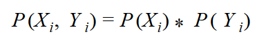
According to the formula, you can calculate an example as follows:

This is the expected probability for independent variables. But we do not see this relationship demonstrated in the combined probabilities recorded in Table 2, which shows a cross-tabulation of X and Y with distributions of X and Y shown on the margins (the rightmost column and the bottommost row) and measured distributions of combined probabilities in the middle cells.
TABLE 2 Combined and marginal probabilities
| X\Y | 1 | 2 | 3 | P(X) |
|---|---|---|---|---|
| 0 | 0.14 | 0 | 0 | 0.14 |
| 1 | 0 | 0.26 | 0.13 | 0.39 |
| 2 | 0 | 0.24 | 0.12 | 0.36 |
| 3 | 0.11 | 0 | 0 | 0.11 |
| P(Y) | 0.25 | 0.50 | 0.25 | 1 \ 1 |
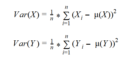
I want to measure the deviation of the actual from the expected probabilities in the intersection cells. Remember the formula for the variance of one variable? Let’s write the formula once again, this time for both variables, X and Y:
First, though, let’s measure the covariance of a variable with itself. We’ll call it Z. Z has only three states (1, 2, and 3). You can imagine an SQL Server table with three rows, one column Z, and a different value in each row. The probability of each value is 0.33, or exactly 1 / (number of rows) —that is, 1 divided by 3. Table 3 shows this variable cross-tabulated with itself. To distinguish between vertical and horizontal representations of the same variable Z, let’s call the variable “Z vertical” and “Z horizontal.”
TABLE 3 One variable cross-tabulated with itself
| Zv\Zh | 1 | 2 | 3 | P(Zv) |
|---|---|---|---|---|
| 1 | 0.33 | 0 | 0 | 0.33 |
| 2 | 0 | 0.33 | 0 | 0.33 |
| 3 | 0 | 0 | 0.33 | 0.33 |
| P(Zh) | 0.33 | 0.33 | 0.33 | 1 \ 1 |
The formula for the variance of a single variable can be expanded to a formula that measures how the variable covaries with itself:
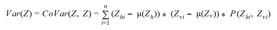
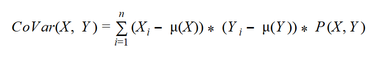
This formula seems suitable for two variables as well. Of course, it was my intention to develop a formula to measure the spread of combined probabilities of two variables. I simply replace one variable —the “horizontal” Z, for example, with X, and the other one (the “vertical” Z) with Y — and get the formula for the covariance:
Calculating the Covariance
Now I can calculate the covariance for two continuous variables, the Age and the YearlyIncome, from the dbo.vTargetMail view from the AdventureWorksDW2014 demo database. I can replace the probability for the combination of the variables P(X, Y) with the probability for each of the n rows combined with itself —that is, with 1 / n2 —and the sum of these probabilities for n rows with 1 / n, because each row has an equal probability. Here is the query that calculates the covariance:
WITH CoVarCTE AS
(
SELECT 1.0*Age as val1,
 AVG(1.0*Age) OVER () AS mean1,
 1.0*YearlyIncome AS val2,
 AVG(1.0*YearlyIncome) OVER() AS mean2
FROM dbo.vTargetMail
)
SELECT
 SUM((val1-mean1)*(val2-mean2)) / COUNT(*) AS Covar
FROM CoVarCTE;
The result of this query is
covar
------------------
53701.023515
To verify whether your result is correct or not, use Correlation Coefficient Calculator to put your data values and get the answer. Covariance indicates how two variables, X and Y, are related to each other. When large values of both variables occur together, the deviations are both positive (because Xi – Mean(X) > 0 and Yi – Mean(Y) > 0), and their product is therefore positive. Similarly, when small values occur together, the product is positive as well. When one deviation is negative and one is positive, the product is negative. This can happen when a small value of X occurs with a large value of Y and the other way around. If positive products are absolutely larger than negative products, the covariance is positive; otherwise, it is negative. If negative and positive products cancel each other out, the covariance is zero. And when do they cancel each other out? Well, you can imagine such a situation quickly—when two variables are really independent. Therefore, the covariance evidently summarizes the relation between variables:
- If the covariance is positive, when the values of one variable are large, the values of the other one tends to be large as well. (positive correlation)
- When the covariance is negative, the values of one variable are large when the values of the other one tends to be small. (negative correlation)
- If the covariance is zero, the variables are independent.
Correlation and Coefficient of Determination
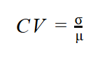
When I derived formulas for the spread of the distribution of a single variable, I wanted to have the possibility of comparing the spread of two or more variables. I had to derive a relative measurement formula—the coefficient of the variation (CV):
Now I want to compare the two covariances computed for two pairs of the variables. Let’s again try to find a similar formula—let’s divide the covariance with something. It turns out that a perfect denominator is a product of the standard deviations of both variables. This is the formula for the correlation coefficient:
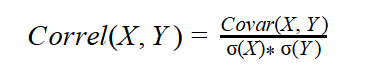
The reason that the correlation coefficient is a useful measure of the relation between two variables is that it is always bounded: –1 <= Correl <= 1. Of course, if the variables are independent, the correlation is zero, because the covariance is zero. The correlation can take the value 1 if the variables have a perfect positive linear relation (if you correlate a variable with itself, for example). Similarly, the correlation would be –1 for the perfect negative linear relation. The larger the absolute value of the coefficient is, the more closely the variables are related. But the significance depends on the size of the sample. A coefficient over 0.50 is generally considered to be significant. However, there could be a casual link between variables as well. To correct the too-large value of the correlation coefficient, it is often squared and thus diminished. The squared coefficient is called the coefficient of determination (CD):
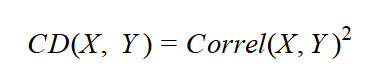
In statistics, when the coefficient of determination is above 0.20, you typically can reject the null hypothesis. In other words, you can say that the two continuous variables are not independent and that, instead, they are correlated. The following query expands the previous one by calculating the correlation coefficient and the coefficient of determination in addition to the covariance.
WITH CoVarCTE AS
(
SELECT 1.0*Age as val1,
 AVG(1.0*Age) OVER () AS mean1,
 1.0*YearlyIncome AS val2,
 AVG(1.0*YearlyIncome) OVER() AS mean2
FROM dbo.vTargetMail
)
SELECT
 SUM((val1-mean1)*(val2-mean2)) / COUNT(*) AS Covar,
 (SUM((val1-mean1)*(val2-mean2)) / COUNT(*)) /
 (STDEVP(val1) * STDEVP(val2)) AS Correl,
 SQUARE((SUM((val1-mean1)*(val2-mean2)) / COUNT(*)) /
 (STDEVP(val1) * STDEVP(val2))) AS CD
FROM CoVarCTE;
The result is
covar          correl                 CD
-------------- ---------------------- ----------------------
53701.023515   0.144329261876658      0.0208309358338609
From the result, you can see that we cannot safely reject the null hypothesis for these two variables. We might have expected a stronger association between the Age and YearlyIncome variables. Let me give you a hint: there is a relationship between these two variables. It is not a simple linear relationship, however. Income increases with age until some point at which it changes direction, thereafter decreasing with age.
Linear Regression
If the correlation coefficient is significant, you know there is some linear relation between the two variables. I would like to express this relation in a functional way—that is, one variable as a function of the other. The linear function between two variables is a line determined by its slope and intercept. The challenge, then, is to identify each of these values. You can quickly imagine that the slope is somehow connected with the covariance.
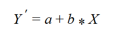
I begin to develop the formula for the slope from another perspective. I start with the formula for the line, where the slope is denoted with b and the intercept with a:
You can imagine that the two variables being analyzed form a two-dimensional plane. Their values define the coordinates of the points in the plane. You are searching for a line that best fits the set of points. Actually, it means that you want the points to fall as close as possible to the line. You need the deviations from the line —that is, the difference between the actual value for Yi and the line value Y’. The following figure shows an example of a linear regression line (the orange line) that best fits the points in the plane. The figure also shows the deviations from the line for three data points.

If you use simple deviations, some are going to be positive and others negative, so the sum of all deviations will be zero for the best-fit line. A simple sum of deviations, therefore, is not a good measure. Squaring the deviations, as we do for the mean squared deviation however, will solve this problem. To find the best-fit line, you must find the lowest possible sum of squared deviations. Here I omit the full derivation, showing instead just the final formulas for the slope and intercept:
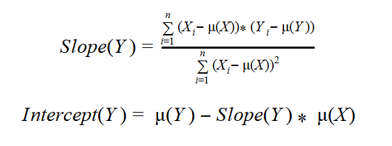
If you look back at the formulas for the covariance and mean squared deviation, you can see that the numerator of the slope really is connected with the covariance, while the denominator closely resembles the mean squared deviation of the independent variable.
During the course of this discussion I have nonchalantly begun using terms such as “independent” (and implicitly) “dependent” variables. How do I know which one is the cause and which one is the effect? Well, in real life it’s usually easy to qualify the roles of the variables. In statistics, just for the purpose of this overview, I can calculate both combinations: Y as function of X, and X as function of Y. Therefore, I get two lines, which are called the first regression line and the second regression line.
After I have the formulas, it is easy to write the queries in T-SQL, as shown in the following query:
WITH CoVarCTE AS
(
SELECT 1.0*Age as val1,
 AVG(1.0*Age) OVER () AS mean1,
 1.0*YearlyIncome AS val2,
 AVG(1.0*YearlyIncome) OVER() AS mean2
FROM dbo.vTargetMail
)
SELECT Slope1=
        SUM((val1 - mean1) * (val2 - mean2))
        /SUM(SQUARE((val1 - mean1))),
       Intercept1=
         MIN(mean2) - MIN(mean1) *
           (SUM((val1 - mean1)*(val2 - mean2))
            /SUM(SQUARE((val1 - mean1)))),
       Slope2=
        SUM((val1 - mean1) * (val2 - mean2))
        /SUM(SQUARE((val2 - mean2))),
       Intercept2=
         MIN(mean1) - MIN(mean2) *
           (SUM((val1 - mean1)*(val2 - mean2))
            /SUM(SQUARE((val2 - mean2))))
FROM CoVarCTE;
The result is
Slope1            Intercept1         Slope2                 Intercept2
----------------  ----------------   --------------------   ----------------------
404.321604291283  37949.8984377112   5.15207092905737E-05   44.9200496725375
Of course, you should understand that this calculation was for the purpose of demonstration only. Because the correlation between these two variables is so low, it would make no sense to calculate the linear regression coefficients in this case.
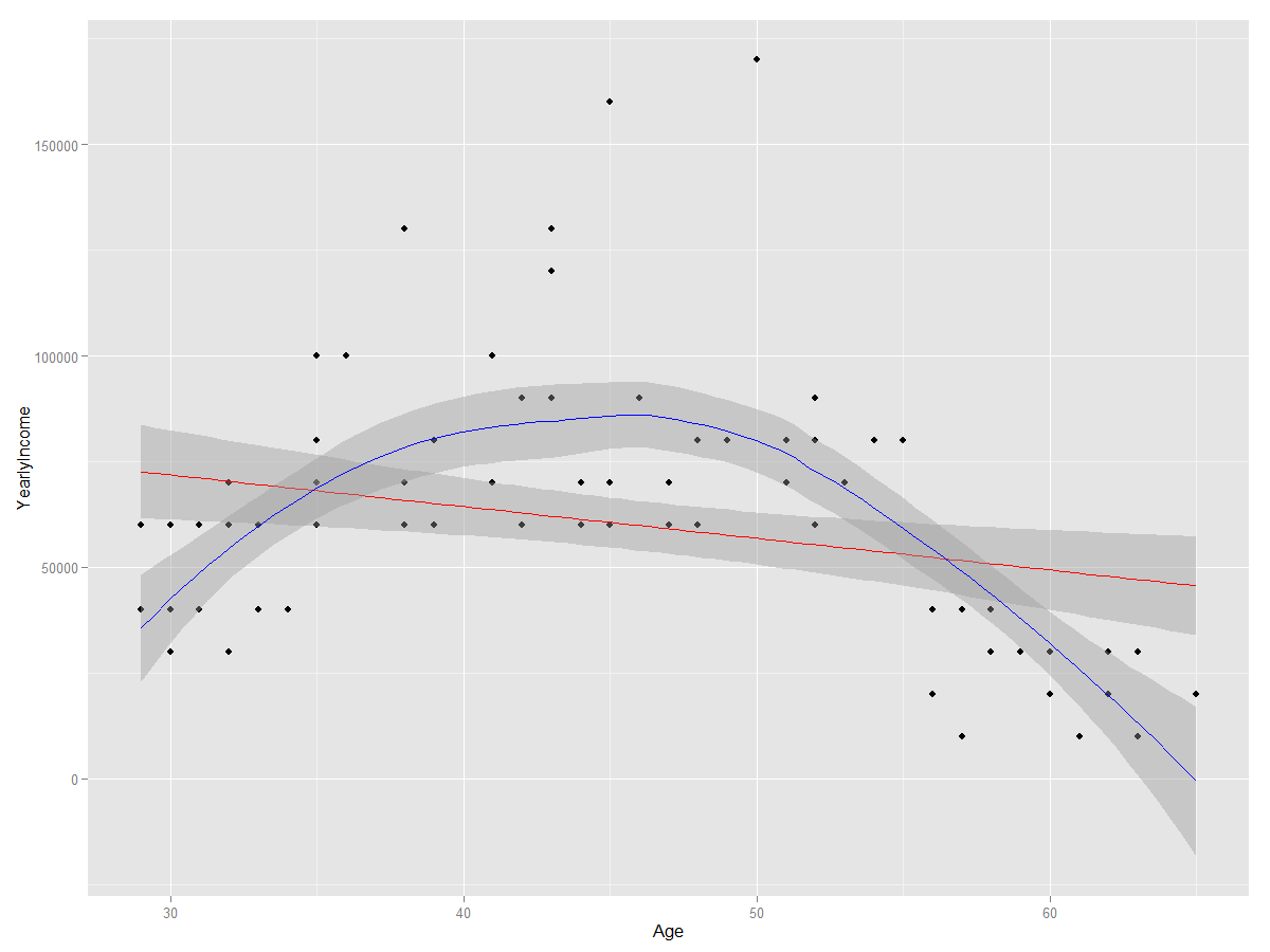
Finally, let me show you the association between age and yearly income in the following graph. The orange line in the graph shows a possible linear association; however, you can see that the line does not fit the data points well. The blue line shows a polynomial association, which is more complex that the linear one, but fits the data points better. It reflects the fact that the income goes up with the age until some point, when the direction of the curve changes, reflecting a decrease in income with any further increase in age. (Note that I created this graph with R, not with T-SQL.)
Conclusion
Before concluding this article, let me point out the common misuse of the correlation coefficient. Correlation does not mean causation. This is a very frequent error. When people see high correlation, they incorrectly infer that one variable causes or influences the values of the other. Again, this is not true. Correlation does not assign cause and effect. In addition, remember that I measure linear dependencies only. Even if the correlation coefficient is zero, this does not mean that the variables are independent (or not related at all). You can say that, if the two variables are independent, they are also uncorrelated, but if they are uncorrelated, they are not necessarily independent.
However, once you understand and know how to calculate the covariance and the correlation coefficient, it is simple to calculate the slope and intercept for the linear regression formula.