Using the Power of the R Language to Query an SQL Database


How do you visualize the results of an SQL query? You usually need to use multiple tools to achieve that. Why not use a tool that communicates with SQL directly and can perform any data analysis task?
R is a data-oriented programming language that uses packages (libraries) to help you with nearly every imaginable data analysis task and more. Some of these packages allow R connect to an SQL database so you can query it and perform any desired action on the result set.
We’ll use a PostgreSQL database with two tables from the Vertabelo Academy SQL Basics course. The two tables are from a section titled How to query more than one table and are named movie and director. As its name suggests, the first table contains information about a few movies and the IDs of their directors. These correspond to the IDs of directors listed in the second table.
I’ll show you how to use the tidyverse suite of packages in R to connect to a database. We’ll execute a couple of queries, get the data into R, and wrap it all up with a visualization.
Every section will have an SQL query on the left and the corresponding R code on the right. I’ll also show you a table with the results from each step.
Connecting to an SQL Database
The first thing to do when communicating with a database from R is to establish a connection. We need to create a connection object that we’ll use in our queries. To do so, we simply use the dbConnect() function from the DBI package.
We need to provide a couple of parameters. The first one is a function that defines the database driver to use. Each database system uses a different driver. For example, PostgreSQL works with the so-called ODBC API (Open Database Connectivity standard).
The last important parameter is the connection string. It defines the address of the database server, the username, the password and the name of the database to which we’d like to connect. The other parameters are optional.
We will be using dplyr to query databases in R. It’s a very popular R package that handles tons of data wrangling tasks and can even communicate with database backends. The best thing about this is that the syntax stays exactly the same—it doesn’t matter if you are wrangling data frames (R’s data format similar to tables) or SQL tables.
Below, you can see how I create a connection object to my SQL database and store it in a variable named con. I also create two connection objects to the movie and director tables and call the variables movie_tbl and director_tbl, respectively. tbl() is a dplyr function that takes a connection object as the first parameter and the table name as the second.
Take a look at the code:
# database connection object
con <- dbConnect(
    odbc::odbc(),
    .connection_string = "
        Driver={PostgreSQL ANSI(x64)};
        Server=127.0.0.1;
        Uid=postgres;
        Pwd=postgres;
        Database=vertabelo;",
    timeout = 10,
    encoding = "windows-1252")

# movie table connection object
movie_tbl <- tbl(con, "movie")

# director table connection object
director_tbl <- tbl(con, "director")
You only have to do the connection part once. After that, you can just enjoy querying the database and getting the results you want.
Now, let’s go step by step from the simplest query to more complex ones that combine multiple tables. We’ll finish it all off with a visualization. All of this will be performed from within the R language!
Selecting All Data from a Table
As promised, we’ll start with a simple example. The simplest SQL query selects everything from one table. Let’s do it, then!
SQL
SELECT * FROM movie
R
movie_tbl
| id | name | year | director_id |
|---|---|---|---|
| 1 | Psycho | 1960 | 1 |
| 2 | Saving Private Ryan | 1998 | 2 |
| 3 | Schindler’s List | 1993 | 2 |
| 4 | Midnight in Paris | 2011 | 3 |
| 5 | Sweet and Lowdown | 1993 | 3 |
| 6 | Pulp fiction | 1994 | 4 |
| 7 | Talk to her | 2002 | 5 |
| 8 | The skin I live in | 2011 | 5 |
Did you notice that we simply wrote the variable name movie_tbl to query the database? The connection itself automatically creates a query to return every column of the table.
Note that calling the variable just prepares the query but doesn’t execute it yet! It will just return a few rows. If we want to execute the query and get all the data, we must call the collect() function.
Selecting Specific Columns from a Table
Let’s incrementally make the query more difficult. I want to show you all the basic SQL keywords and their R equivalents.
Here comes the R language and its select() function. It allows us to specify what columns we actually want to retrieve from a table. In SQL, you’d replace the asterisk with the column names. We’ll only select the name and year columns from the movie table here.
SQL
SELECT name, year
FROM movie
R
movie_tbl %>%
    select(name, year)
| name | year |
|---|---|
| Psycho | 1960 |
| Saving Private Ryan | 1998 |
| Schindler’s List | 1993 |
| Midnight in Paris | 2011 |
| Sweet and Lowdown | 1993 |
| Pulp fiction | 1994 |
| Talk to her | 2002 |
| The skin I live in | 2011 |
The R code literally says to connect to a table named movie and select the name and year columns. That’s practically an English sentence, right?
The odd thing you may have noticed is the so-called pipe operator, or %>%. It simplifies the code and makes it more readable. The pipe helps us maintain a logical flow, passing along data from one part of the query to the next. Its role should become clear once we add more pipes later. Simply think of the pipe as the English word then.
Filtering Selected Data from a Table
Selecting our desired columns is a good start. But we might have a lot of rows in our database and may only be interested in returning a certain subset. For example, what if we only want to see movies that were made after the year 1993?
SQL
SELECT name, year
FROM movie
WHERE year > 1993
R
movie_tbl %>%
    select(name, year) %>%
    filter(year > 1993)
| name | year |
|---|---|
| Saving Private Ryan | 1998 |
| Midnight in Paris | 2011 |
| Pulp fiction | 1994 |
| Talk to her | 2002 |
| The skin I live in | 2011 |
In SQL, you’d simply do this with the WHERE keyword and the condition you want to meet. In the R language, we pipe our previous query to the filter() function. The condition we specify is the same—only the keyword changes.
Sorting Data from a Table
Now that we have a set of movies released after 1993, we may want to ensure that they’re sorted in a specific way.
SQL
SELECT name, year
FROM movie
WHERE year > 1993
ORDER BY year
R
movie_tbl %>%
    select(name, year) %>%
    filter(year > 1993) %>%
    arrange(year)
| name | year |
|---|---|
| Pulp fiction | 1994 |
| Saving Private Ryan | 1998 |
| Talk to her | 2002 |
| Midnight in Paris | 2011 |
| The skin I live in | 2011 |
Here, we sorted the movies by year. SQL allows us to do this with the ORDER BY clause followed by the name of a column (or columns) by which we want to sort the data.
R actually isn’t that different. It just uses different keywords. In R, we arrange() tables and specify the column names as function arguments. See how we used the code from the previous part but just added the pipe %>% to forward the result to the next part of the query?
Joining Two Tables
One single table rarely contains enough information for performing proper data analysis. We know that each of our movies has a director_id. But that doesn’t tell us much. It would be a lot more informative to see the names of the movie directors, or even some more columns.
Let’s join these two tables to see who directed what. We’ll be using a LEFT JOIN just in case a movie doesn’t have a value in the director_id column (all of them do, though).
SQL
SELECT movie.*,
       director.name AS director_name
FROM movie
LEFT JOIN director
ON (movie.director_id = director.id)
R
movie_tbl %>%
    left_join(director_tbl,
    by = c("director_id" = "id")) %>%
    rename(director_name = name.y)
| id | name.x | year | director_id | director_name | birth_year |
|---|---|---|---|---|---|
| 1 | Psycho | 1960 | 1 | Alfred Hitchcock | 1899 |
| 2 | Saving Private Ryan | 1998 | 2 | Steven Spielberg | 1946 |
| 3 | Schindler’s List | 1993 | 2 | Steven Spielberg | 1946 |
| 4 | Midnight in Paris | 2011 | 3 | Woody Allen | 1935 |
| 5 | Sweet and Lowdown | 1993 | 3 | Woody Allen | 1935 |
| 6 | Pulp fiction | 1994 | 4 | Quentin Tarantino | 1963 |
| 7 | Talk to her | 2002 | 5 | Pedro Almodóvar | 1949 |
| 8 | The skin I live in | 2011 | 5 | Pedro Almodóvar | 1949 |
To each of our movies, we LEFT JOIN a director. In SQL, we specify the columns on which we want to join these two tables using the ON clause. The R code is once again very similar—we take the movie table and pipe it to the left_join() function with the director table as the first argument. Instead of the ON statement in SQL, we specify a vector for the by parameter.
We also do a little bit of renaming here using the rename() function. That’s because both of our tables have column named name. R automatically suffixes the column names with .x and .y and still executes the query. SQL might complain about ambiguous column names. We know that the name.y column is actually the name of the director, so we rename it to director_name.
Creating a New Column
There are often times when you need to create new columns on the fly. That usually happens when you don’t want to create columns for data that can be easily computed at runtime.
We have such a case here. What if we would like to know how old each director was when they directed their movie?
SQL
SELECT movie.*,
       director.name AS director_name,
       (movie.year - director.birth_year) AS director_age
FROM movie
LEFT JOIN director
ON (movie.director_id = director.id)
R
movie_tbl %>%
    left_join(director_tbl,
    by = c("director_id" = "id")) %>%
    rename(director_name = name.y) %>%
    mutate(director_age = year - birth_year)
| id | name.x | year | director_id | director_name | birth_year | director_age |
|---|---|---|---|---|---|---|
| 1 | Psycho | 1960 | 1 | Alfred Hitchcock | 1899 | 61 |
| 2 | Saving Private Ryan | 1998 | 2 | Steven Spielberg | 1946 | 52 |
| 3 | Schindler’s List | 1993 | 2 | Steven Spielberg | 1946 | 47 |
| 4 | Midnight in Paris | 2011 | 3 | Woody Allen | 1935 | 76 |
| 5 | Sweet and Lowdown | 1993 | 3 | Woody Allen | 1935 | 58 |
| 6 | Pulp fiction | 1994 | 4 | Quentin Tarantino | 1963 | 31 |
| 7 | Talk to her | 2002 | 5 | Pedro Almodóvar | 1949 | 53 |
| 8 | The skin I live in | 2011 | 5 | Pedro Almodóvar | 1949 | 62 |
We need to join the tables again, of course. In SQL, we need to create a new column in a SELECT statement. We called it director_age, and it’s the difference between a movie’s release year and its director’s birth year.
The R language introduces one more important function for this purpose: mutate(). This creates one or more new columns based on other columns in the selected data. Creating new columns in R is arguably far more straightforward; you just need to pipe the query to the function again.
Data Visualization in R
For this upcoming last section, assume that we stored the above R code in a variable named directors. We’ll use that variable to create a simple data visualization.
After you select and wrangle all the data you need, the best way to understand the data is often to visualize it. I’ll show you how to create a histogram of director ages.
Bear in mind that the dataset we’ve been working with is small, so the plot might not be as helpful or visually appealing as it would be if it were to contain thousands of records.
ggplot(directors, aes(director_age)) +
    geom_histogram(binwidth = 20, fill = "#592a88") +
    labs(
        title = "Histogram of director's ages",
        x = "Director age",
        y = "Count"
    )
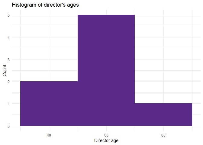
We can see the rough age distribution here in the histogram. As soon as we get the data ready, we can start visualizing it right away—we don’t need to export anything anywhere. We don’t even need to use a different tool. R provides everything we need!
Summary
I showed you how simple SQL SELECT queries can be translated to R code and vice versa. Both languages use commands that resemble English sentences, which makes it much easier to write queries.
I especially wanted to emphasize that once you get the data ready, you can start doing powerful analyses and/or visualizations right away—there’s very little, if any, prep work involved.
If you want to play with the code from this article yourself, take a look at my GitHub repo.
Thanks for reading!