Ever wondered how you can use Python to create stunning data visualizations?

In the first part of this series, we saw how to draw line plots and histograms using the matplotlib library. We also saw how to change the default size of a plot and how to add titles, axes, and legends to a plot.

In this article, we’ll see a few more types of plots that can be drawn using the matplot library with pro tips on how to improve them. We’ll cover the following plots:

• Bar plots
• Scatter plots
• Stack plots
• Pie plots

As a quick reminder, we’ll be using the alias of plt for the matplotlib module in our code. Thus, all matplotlib function calls will be preceded by plt.

Let’s dive right in!

Bar plots

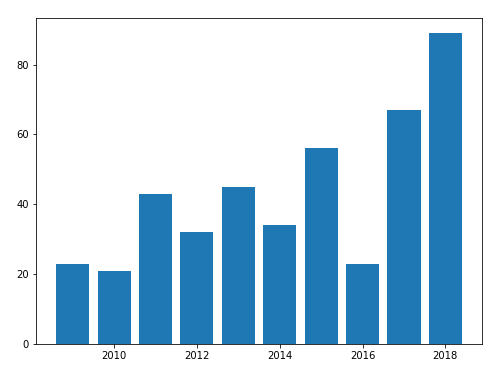
A bar plot simply uses a bar to represent the y-value for a particular x-value. For instance, you could use a bar plot to depict the stock prices over the past ten years. To do so, you’d use the bar function. The first argument to this function is the list of values for the x-axis, and the second argument is the list of corresponding values for the y-axis. It’s important to mention that the number of points in the x and y lists must be equal.

Consider the following script:

stock_prices = [23,21,43,32,45,34,56,23,67,89]
years = [2009, 2010, 2011, 2012, 2013, 2014, 2015, 2016, 2017, 2018] 

plt.bar(years, stock_prices)
plt.show()

The output looks like this:

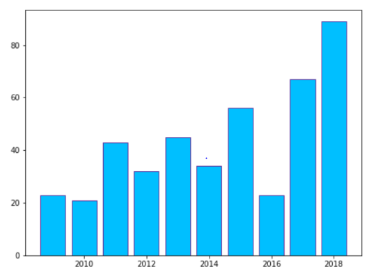
You can change the color of the bars by passing in a value to the color parameter of the bar function, as shown below:

stock_prices = [23,21,43,32,45,34,56,23,67,89]
years = [2009, 2010, 2011, 2012, 2013, 2014, 2015, 2016, 2017, 2018] 

plt.bar(years, stock_prices, color = "deepskyblue", edgecolor = "rebeccapurple")
plt.show()

In the above script, the value of the color attribute is set to deepskyblue. The output of the script above looks like this:

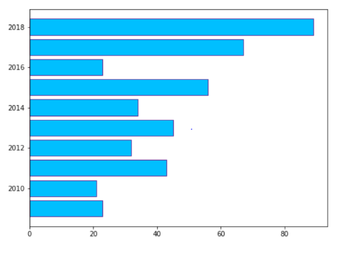
Pro Tip: How to Create Horizontal Bar Plots

In addition to vertical bar graphs, you can also draw horizontal bar graphs. To do so, you simply need to pass in horizontal as the value for the orientation parameter of the bar function. Look at the following script:

stock_prices = [23,21,43,32,45,34,56,23,67,89]
years = [2009, 2010, 2011, 2012, 2013, 2014, 2015, 2016, 2017, 2018] 

plt.barh(years, stock_prices, orientation = "horizontal", color = "deepskyblue", edgecolor = "rebeccapurple")
plt.show()

In the output, you will see a horizontal bar plot as shown below:

Scatter Plots

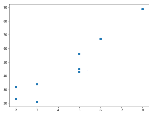
Scatter plots are similar to line plots, but they don’t use curves to show a relationship between the values of the x- and y-axes. Instead, you simply plot each pair of x and y values. To create a scatter plot, you simply need to use the scatter function. The values for the x- and y-axes are passed in as the first and second arguments to this function, respectively.

Look at the following script:

stock_prices = [23,21,43,32,45,34,56,23,67,89,23,21,43,32,45,34,56,23,67,89,23,21,43,32,45,34,56,23,67,89]
credit_ratings = [2,3,5,2,5,3,5,2,6,8,2,3,5,2,5,3,5,2,6,8,2,3,5, 2,5,3,5,2,6,8] 

plt.scatter(credit_ratings, stock_prices)
plt.show()

The output of the script above looks like this:

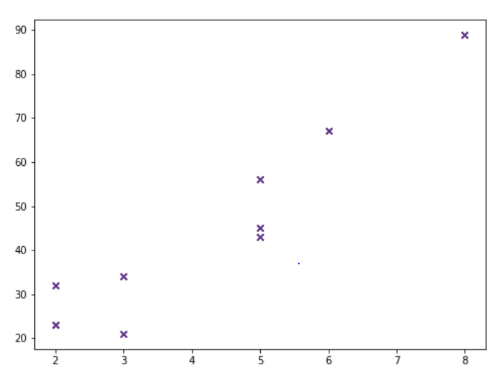
By default, blue circles are used for scatter plots, but you can change the shape and color. The shape to be drawn is specified by the marker parameter. Similarly, the plot color is passed in to the color parameter. Look at the following script:

stock_prices = [23,21,43,32,45,34,56,23,67,89,23,21,43,32,45,34,56,23,67,89,23,21,43,32,45,34,56,23,67,89]
credit_ratings = [2,3,5,2,5,3,5,2,6,8,2,3,5,2,5,3,5,2,6,8,2,3,5, 2,5,3,5,2,6,8] 

plt.scatter(credit_ratings, stock_prices, marker = "x", color = "#5d3087")
plt.show()

Here, ‘x’ is passed in as the marker, while the hex code #5d3087 is passed in as the color. Alternatively, you could pass in the name of the color instead of its hex value. The output of the script above looks like this:

Pro Tip: How to Change the Marker Size for Scatter Plots

You can change the default size of the marker on a scatter plot by passing in a value for the s parameter. The default value is 20. Look at the following script:

stock_prices = [23,21,43,32,45,34,56,23,67,89,23,21,43,32,45,34,56,23,67,89,23,21,43,32,45,34,56,23,67,89]
credit_ratings = [2,3,5,2,5,3,5,2,6,8,2,3,5,2,5,3,5,2,6,8,2,3,5, 2,5,3,5,2,6,8] 

plt.scatter(credit_ratings, stock_prices, marker = "o", color = "deepskyblue", edgecolors = "rebeccapurple", s = 400)
plt.show()

The output looks like this:

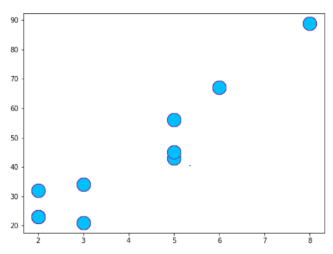
Of course, as you can probably tell, these markers are quite large and make it a little difficult to tell what values they correspond to on the x- and y-axes. This was more of an illustrative exercise. When producing your own scatter plots, be sure to select a reasonable marker size that balances visibility with clarity.

Stack Plots

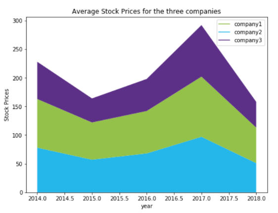
Stack plots are used when you have data from multiple categories for each data point of the x-axis. For instance, you can use the stack plot to plot the stock prices for three companies over the past eight years. The data for the companies will be stacked on top of each other to make it easier to compare them.

To draw a stack plot, you need to use the stackplot function of the plt module. The first argument is the list of data to be plotted on the x-axis, while the rest of the arguments are the data for each category that you want in your stack plot. You can also specify the color for each stack using the color attribute.

year = [2014, 2015, 2016, 2017, 2018]

company1 = [78,57,68,97,51]  
company2 = [85,65,74,105,62]  
company3 = [65,42,56,90,45]

plt.plot([],[], color = "#93c149", label = "company1")  
plt.plot([],[], color = "#25b6ea", label = "company2")  
plt.plot([],[], color = "#5d3087", label = "company3")

plt.stackplot(year,company1,company2,company3,colors = ["#25b6ea","#93c149","#5d3087"])  

plt.legend()  
plt.title("Average Stock Prices for the three companies")  
plt.xlabel("year")  
plt.ylabel("Stock Prices")  
plt.show()

The output of the script above looks like this:

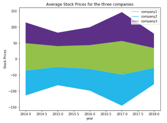
Pro Tip: How to Create Symmetric Stack Plots

You can also create symmetrical stack plots by passing in ‘sym’ as the value for the baseline parameter, as shown below:

year = [2014, 2015, 2016, 2017, 2018]

company1 = [78,57,68,97,51]  
company2 = [85,65,74,105,62]  
company3 = [65,42,56,90,45]

plt.plot([],[], color = "#93c149", label = "company1")  
plt.plot([],[], color = "#25b6ea", label = "company2")  
plt.plot([],[], color = "#5d3087", label = "company3")

plt.stackplot(year, company1, company2, company3, colors = ["#25b6ea","#93c149","#5d3087"] , baseline = "sym")  

 
plt.legend()  
plt.title("Average Stock Prices for the three companies")  
plt.xlabel("year")  
plt.ylabel("Stock Prices")  
plt.show()

In the output, you’ll see a symmetrical stack plot:

Pie Plots

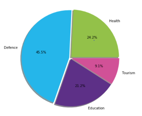
Pie plots are in the form of a circle, where each slice represents the portion of data that belongs to that specific category. To draw a pie plot, you need to call the pie function of the plt module. The first argument is the list of data. You then need to pass in the list of category names to the labels parameter. If the shadow parameter is set to True, a thin shadow appears near the edges of the chart. Finally, the explode parameter can be used to add space between the different slices of the pie plot.

It’s important to mention that you do not have to specify the exact percentage that each category will occupy on the plot. Rather, you simply need to specify the value for each category; the pie plot will automatically convert these to percentages. The following script creates a pie plot for the imaginary budget spending of a country for one year:

sectors = "Health", "Defence", "Education', "Tourism"

amount = [40,75,35,15]  
colors = ["#93c149","#25b6ea","#5d3087","#d15197"]

plt.pie(amount, labels = sectors, colors = colors ,shadow = True, explode = (0.025, 0.025, 0.025, 0.025), autopct = "%1.1f%%")  
plt.axis("equal")

plt.show()

The output of the script looks like this:

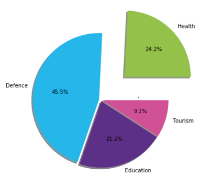
Let’s increase the explode value for the first category and see what results we get. We’ll set it to 0.5:

sectors = "Health", "Defence", "Education", "Tourism"

amount = [40,75,35,15]  
colors = ["#93c149","#25b6ea","#5d3087","#d15197"]

plt.pie(amount, labels = sectors, colors=colors ,shadow = True, explode = (0.5, 0.025, 0.025, 0.025), autopct = "%1.1f%%")  
plt.axis("equal")

plt.show()  

In the output, you’ll see an increased distance between Health and the other categories, as shown below:

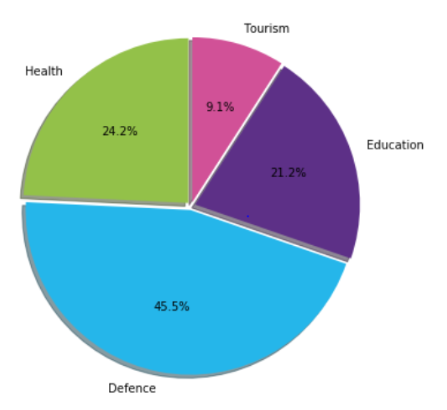
Pro Tip: Changing Angles with Respect to the Baseline

By default, the slices of a pie plot are arranged such that the category with the largest share of the plot will appear in the top-left corner, and the others in random locations. However, you can change this behavior.

For instance, if you want your first category to have a 90-degree angle with respect to the baseline (an imaginary horizontal line passing through the center of the pie), you can pass in 90 as the value for the startangle parameter of the pie function, as shown below:

sectors = "Health", "Defence", "Education", "Tourism"

amount = [40,75,35,15]  
colors = ["#93c149","#25b6ea","#5d3087","#d15197"]

plt.pie(amount, labels = sectors, colors = colors ,shadow = True, explode = (0.025, 0.025, 0.025, 0.025), autopct = "%1.1f%%", startangle = 90)  
plt.axis('equal')

plt.show()  

In the output, you’ll see that the category named Health now has an angle of 90 degrees with respect to the baseline:

Conclusion

That about wraps it up!

In this article, you learned how to draw bar plots, stack plots, scatter plots, and pie plots. The matplotlib library is a must-have for anyone interested in learning how to plot and visualize data.

Want to learn more about data visualization with matplotlib? Be sure to check out our Introduction to Python for Data Science course. It’s an excellent resource for both beginners and intermediate Python users who want to learn more about data science and data visualization in Python.