High-Performance Statistical Queries: Dependencies Between Continuous and Discrete Variables


In my previous articles, I explained how you can check for associations between two continuous and two discrete variables. This time, we’ll check for linear dependencies between continuous and discrete variables. You can do this by measuring the variance between the means of the continuous variable and different groups of the discrete variable. The null hypothesis here is that all variances between the means are a result of the variance within each group. If you reject this null hypothesis, then there is some significant variance in the means between the groups. This is also known as the residual, or unexplained, variance. You are analyzing the variance of the means, so this is known as an analysis of variance, or ANOVA.

Introducing ANOVA
Intuitively, you would expect that people who have more cars also have a higher income. But that isn’t always the case. For example, the founder of IKEA, Ingvar Kamprad, was living a very modest life and drove a single car—an inexpensive Volvo—but his income was very high.
Now, imagine that Mr. Kamprad somehow appears in your sample of 18,484 people. You have data about each person’s yearly income and the number of cars they own. The number of cars a person owns is a discrete variable with possible values ranging from 0 to 4 (these odd numbers are from a demo that I’ll show later). You calculate the average income for each group based on the number of cars owned—that is, for each category of the discrete variable.
Suddenly, you realize that people with a single car are by far the wealthiest. Is this true? Being the astute statistician that you are, you notice that this comes from the variability within the group of 0 cars, not because of the variability between the groups.
As a quick example, the following graph shows a box-and-whisker plot of the continuous YearlyIncome variable in each of the groups of the NumberCarsOwned discrete variable, both taken from the dbo.vTargetMail view of the AdventureWorksDW demo database.
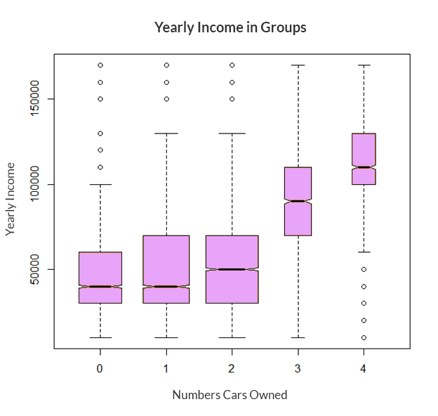
The notched line in each box represents the median of the YearlyIncome in each class of NumberCarsOwned. The top border of each box is the third quartile for each group, and the bottom border is the first quartile for each group. Thus, the height of each box represents the interquartile range (IQR) for that group. The horizontal lines above and below each box (connected with vertical dashed lines) represent the limits of the regular values, or the whiskers of each box, and are at 1.5 times the interquartile range above the upper quartile and below the lower quartile. Outside these whiskers, outliers are represented with small, open circles.
You calculate the variance between groups (MSA) as the sum of squares of deviations of the group mean ( μi ) from the total mean ( µ ) multiplied by the number of cases in each group (ni), with the degrees of freedom equal to the number of groups (a) minus one. The formula is:
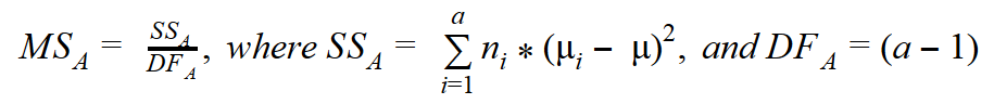
The discrete variable has a finite number of states; µ is the overall mean of the continuous variable; and µi is the mean of the continuous variable in the ith group of the discrete variable.
You start calculating the variance within groups (MSE) by calculating the squares of deviations of individual values from the group mean (e.g., calculating the squares of deviations of individual values in the group with 0 cars from the mean for the group with 0 cars). Then, you sum all the squares in each group separately. Finally, you sum the squares again, this time across all groups. The degrees of freedom are equal to the sum of the number of rows in each group minus one:
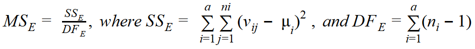
In the above equations, vij denotes the individual value of the continuous variable (YearlyIncome) for a particular discrete category (NumberCarsOwned). Additionally, µi denotes the mean of the continuous variable in the ith group of the discrete variable, and ni denotes the number of observations in the ith group of the discrete variable.
Once you’ve calculated variances within and between the groups, you can then calculate the F ratio as the ratio of the variance between the groups and the variance within the groups:

A large F value means you can reject the null hypothesis. Tables for the cumulative distribution under the tails of F distributions for different degrees of freedom are already calculated. For a specific F value with degrees of freedom between groups and degrees of freedom within groups, you can get critical points where there is, for example, a less than 5% of distribution under the F distribution curve up to or from the specific F point. This means that there is a less than 5% probability that the null hypothesis is correct (that is, there is an association between the means and the groups). If you get a large F value when splitting or sampling your data, this suggests that the splitting or sampling was not random.
You can see the F probability density function in the following figure:
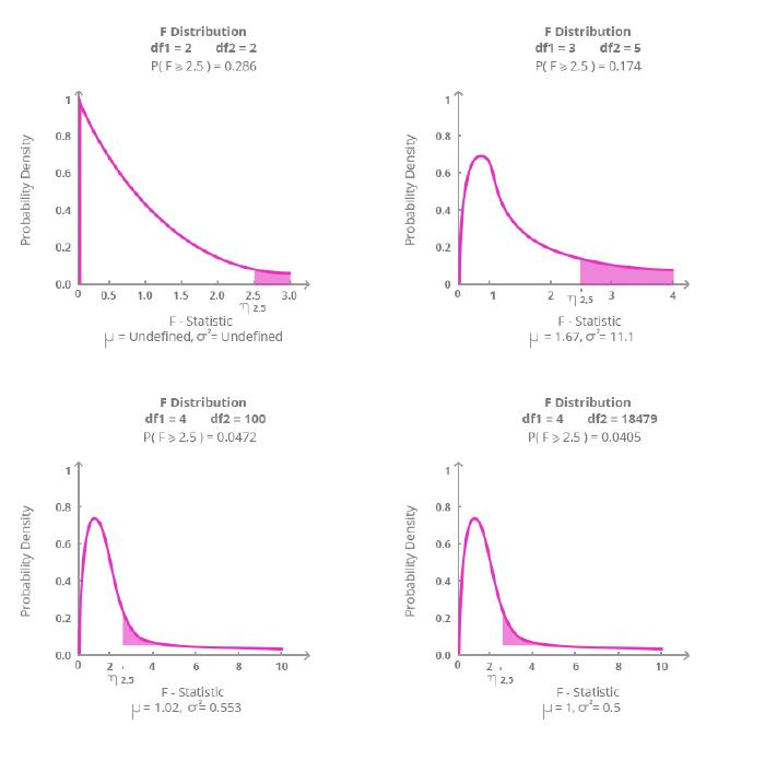
The figure shows F functions for different degrees of freedom with the probability from F = 2.5. I created this graph in the R programming language using the visualize.f() function from the visualize package.
If you look at the graphs of the F distribution for different degrees of freedom, you can see the amount of distribution under the F curve (the blue area) from the specific point of F = 2.5. For example, in the top-right graph, you can see that for the degrees of freedom equal to 3 and 5, there is a 17.4% distribution to the right of the point F = 2.5.
Calculating the F Ratio
You could use the F value to search the F distribution tables and determine whether the two variables (YearlyIncome and NumberCarsOwned) are associated at a particular significance level. However, I want to show how you can calculate the F probability on the fly. It’s quite simple to calculate the cumulative F distribution using CLR code (for example, with a C# application).
Unfortunately, the CLR FDistribution method is implemented in a class that is not supported by SQL Server. However, you can create a console application and then call it from SQL Server Management Studio using the SQLCMD mode.
In Visual Studio, you first create a new Visual C# console application. Then, you need to add a reference to System.Windows.Forms.DataVisualization. And then, you simply write the C# code that calculates the cumulative F distribution:
using System;
using System.Windows.Forms.DataVisualization.Charting;

class FDistribution
{
    static void Main(string[] args)
    {
        // Test input arguments
        if (args.Length != 3)
        {
            Console.WriteLine("Please use three arguments: double FValue, int DF1, int DF2.");
            //Console.ReadLine();
            return;
        }

        // Try to convert the input arguments to numbers.
        // FValue
        double FValue;
        bool test = double.TryParse(args[0], System.Globalization.NumberStyles.Float,
             System.Globalization.CultureInfo.InvariantCulture.NumberFormat, out FValue);
        if (test == false)
        {
            Console.WriteLine("First argument must be double (nnn.n).");
            return;
        }

        // DF1
        int DF1;
        test = int.TryParse(args[1], out DF1);
        if (test == false)
        {
            Console.WriteLine("Second argument must be int.");
            return;
        }

        // DF2
        int DF2;
        test = int.TryParse(args[2], out DF2);
        if (test == false)
        {
            Console.WriteLine("Third argument must be int.");
            return;
        }

        // Calculate the cumulative F distribution function probability
        Chart c = new Chart();
        double result = c.DataManipulator.Statistics.FDistribution(FValue, DF1, DF2);
        Console.WriteLine("Input parameters: " +
            FValue.ToString(System.Globalization.CultureInfo.InvariantCulture.NumberFormat)
            + " " + DF1.ToString() + " " + DF2.ToString());
        Console.WriteLine("Cumulative F distribution function probability: " +
            result.ToString("P"));
    }
}
Calculating the One-Way ANOVA
The following query performs the one-way ANOVA, the analysis of variance using one input discrete variable (the NumberCarsOwned variable) and the YearlyIncome continuous variable from the dbo.vTargetMail view of the AdventureWorksDW demo database:
WITH Anova_CTE AS
(
SELECT NumberCarsOwned, YearlyIncome,
 COUNT(*) OVER (PARTITION BY NumberCarsOwned) AS gr_CasesCount,
 DENSE_RANK() OVER (ORDER BY NumberCarsOwned) AS gr_DenseRank,
 SQUARE(AVG(YearlyIncome) OVER (PARTITION BY NumberCarsOwned) -
        AVG(YearlyIncome) OVER ()) AS between_gr_SS,
 SQUARE(YearlyIncome -
        AVG(YearlyIncome) OVER (PARTITION BY NumberCarsOwned))
		AS within_gr_SS
FROM dbo.vTargetMail
)
SELECT N'Between groups' AS [Source of Variation],
 SUM(between_gr_SS) AS SS,
 (MAX(gr_DenseRank) - 1) AS df,
 SUM(between_gr_SS) / (MAX(gr_DenseRank) - 1) AS MS,
 (SUM(between_gr_SS) / (MAX(gr_DenseRank) - 1)) /
 (SUM(within_gr_SS) / (COUNT(*) - MAX(gr_DenseRank))) AS F
FROM Anova_CTE
UNION
SELECT N'Within groups' AS [Source of Variation],
 SUM(within_gr_SS) AS SS,
 (COUNT(*) - MAX(gr_DenseRank)) AS df,
 SUM(within_gr_SS) / (COUNT(*) - MAX(gr_DenseRank)) AS MS,
 NULL AS F
FROM Anova_CTE;
The query uses a bit of creativity to calculate the degrees of freedom. It calculates the degrees of freedom between groups by calculating the dense rank of the groups and subtracting 1. The dense rank has the same value for all rows belonging to the same group. By finding the maximum dense rank, you can find the number of groups.
The query also calculates the degrees of freedom within groups as the total number of cases minus the number of groups. This way, everything can be calculated with a single scan of the data in the common table expression and in the outer query that refers to the common table expression.
The outer query actually consists of two queries with unioned result sets. This is not necessary from the query perspective, and it might even be less efficient than a single query. However, I chose to use two unioned result sets to get the output that follows the standard statistical way of presenting ANOVA results. Here is the output of the query:
| Source of Variation | SS | df | MS | F |
|---|---|---|---|---|
| Between groups | 6321848616821.04 | 4 | 1580462154205.26 | 2256.21946654061 |
| Within groups | 12944379117665.6 | 18479 | 700491320.832602 | NULL |
The last thing to do is check the significance level of the F value for the specified degrees of freedom. I deployed the FDistribution.exe console application to the C:\temp folder. In SQL Server Management Studio, you can enable the SQLCMD mode in the Query menu. Then, you can execute the following command:
!!C:\StatisticalQueries\FDistribution 7.57962783966074 7 2147
With these input parameters, which are the result of the ANOVA query we ran earlier, you’ll get the following result:
Input parameters: 2256.21946654061 4 18479
Cumulative F distribution function probability: 0.00 %
This means that there is a less than 0.00% probability that the two variables are independent. Of course, you know that this is true in real life—people with more cars do tend to have a higher income!
Conclusion
Now, you know how to check for dependencies between different kinds of variables—two continuous and two discrete, as well as one discrete and one continuous. In this and my previous six articles, I have shown how you can use T-SQL to calculate quite a few basic statistical measures as well as advanced. In the future, I plan to move away from statistics and talk about some other interesting topics, such as how you can calculate definite integration and moving averages with T-SQL.