Visualizing Time Series Data with the Python Pandas Library


How can Python’s pandas library be used to analyze time series data? Let’s find out.
The pandas library is frequently used to import, manage, and analyze datasets in a variety of formats. In this article, we’ll use it to analyze Microsoft’s stock prices for previous years. We’ll also see how to perform basic tasks, such as time resampling and time shifting, with pandas.
What is Time Series Data?
Time series data contains values dependent on some sort of time unit. The following are all examples of time series data:
- The number of items sold per hour during a 24-hour period
- The number of passengers who travel during a one-month period
- The price of stock per day
In all of these, the data is dependent on time units; in a plot, time is presented on the x-axis and the corresponding data values are presented on the y-axis.
Getting the Data
We’ll be using a dataset containing Microsoft’s stock prices for 2013 to 2018. The dataset can be freely downloaded from Yahoo Finance. You may need to enter the time span to download the data, which will arrive in the CSV format.
Importing the Required Libraries
Before you can import the dataset into your application, you will need to import the required libraries. Execute the following script to do so.
import numpy as np
import pandas as pd

%matplotlib inline
import matplotlib.pyplot as plt
This script imports the NumPy, pandas, and matplotlib libraries. These are the libraries needed to execute the scripts in this article.
Note: All the scripts in the dataset have been executed using the Jupyter notebook for Python.
Importing and Analyzing the Dataset
To import the dataset, we will use the read_csv() method from the pandas library. Execute the following script:
stock_data = pd.read_csv('E:/Datasets/MSFT.csv')
To see how the dataset looks, you can use the head() method. This method returns the first five rows of the dataset.
stock_data.head()
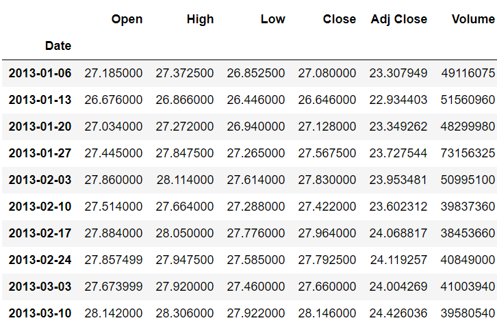
The output looks like this:
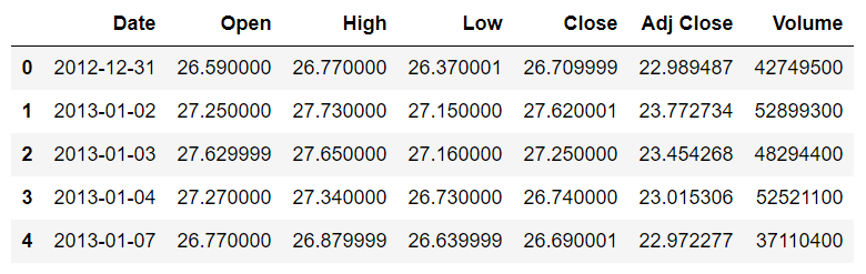
You can see that the dataset contains the date and the opening, high, low, closing and adjusted closing prices for the Microsoft stock. At the moment, the Date column is being treated as a simple string. We want the values in the Date column to be treated as dates. To do so, we need to convert the Date column to the datetime type. The following script does that:
stock_data['Date'] = stock_data['Date'].apply(pd.to_datetime)
Finally, we need the Date column to be used as an index column, since all the other columns depend upon the values in this column. To do this, execute the following script:
stock_data.set_index('Date',inplace=True)
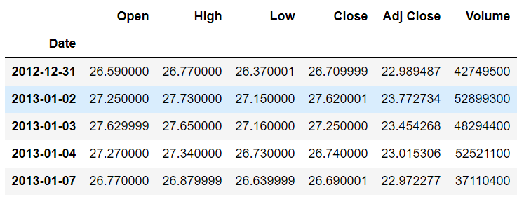
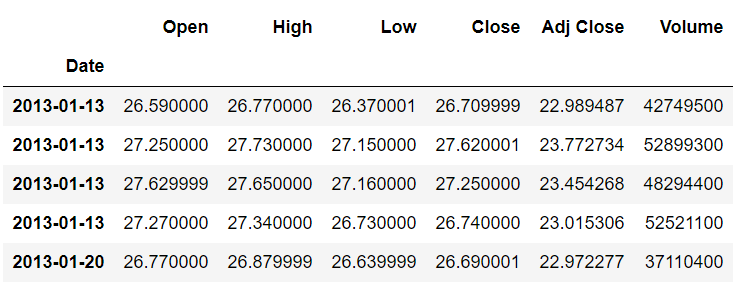
If you use the head() method again, you will see that the values in the Date column are bolded, as shown in the following image. This is because the Date column is now being treated as the index column:
Now, let’s plot the values from the Open column against the date. To do this, execute the following script:
plt.rcParams['figure.figsize'] = (10, 8)   # Increases the Plot Size
stock_data['Open'].plot(grid = True)
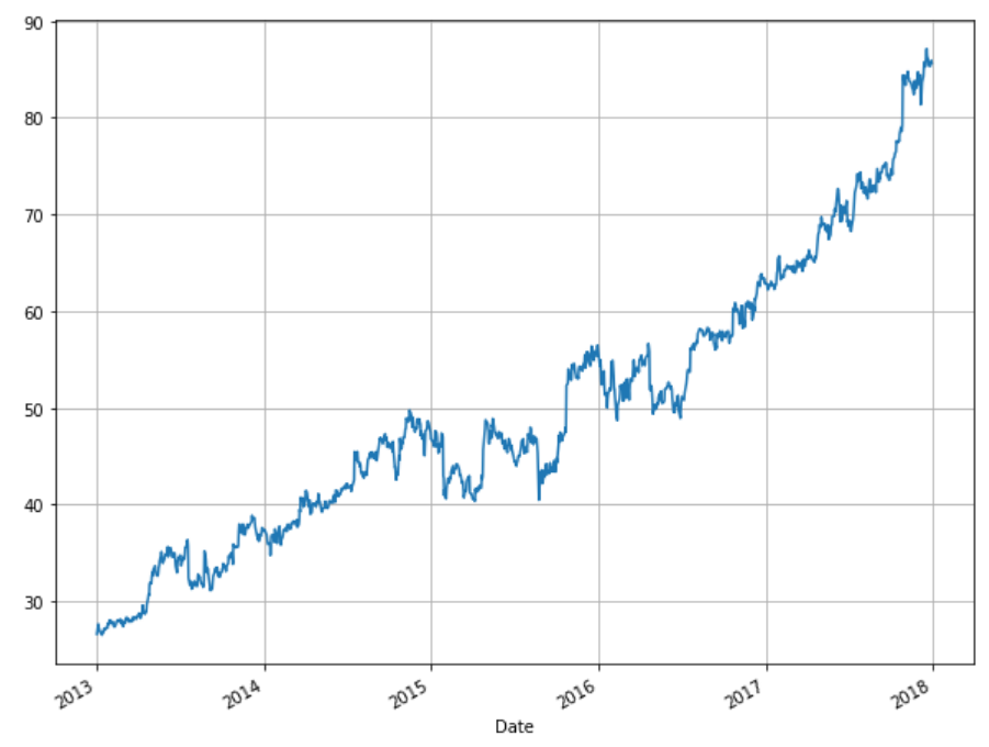
The output shows the opening stock prices from January 2013 to the end of 2017:

Next, we’ll use the pandas library for time resampling. If you need to refresh your pandas, matplotlib, or NumPy skills before continuing, check out Vertabelo Academy’s Introduction to Python for Data Science course.
Time Resampling
Time resampling refers to aggregating time series data with respect to a specific time period. By default, you have stock price information for each day. What if you want to get the average stock price information for each year? You can use time resampling to do this.
The pandas library comes with the resample() function, which can be used for time resampling. All you have to do is set an offset for the rule attribute along with the aggregation function(e.g. maximum, minimum, mean, etc).
Following are some of the offsets that can be used as values for the rule attribute of the resample() function:
W       weekly frequency
M       month end frequency
Q       quarter end frequency
A       year end frequency
The complete list of offset values can be found in the pandas documentation.
Now you have all the information you need for time resampling. Let’s implement it. Suppose you want to find the average stock prices for all the years. To do this, execute the following script:
stock_data.resample(rule='A').mean()
The offset value ‘A’ specifies that you want to resample with respect to the year. The mean() function specifies that you want to find the average stock values.
The output looks like this:
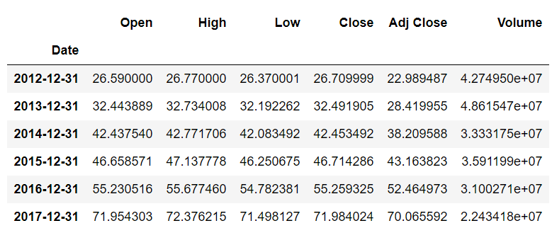
You can see that the value for the Date column is the last day of that year. All the other values are the mean values for the whole year.
Similarly, you can find the average weekly stock prices using the following script. (Note: The offset for week is ‘W’.)
stock_data.resample(rule='W').mean()
Output:
Using Time Resampling to Plot Charts
You can also plot charts for a specific column using time resampling. Look at the following script:
plt.rcParams['figure.figsize'] = (8, 6) # change plot size
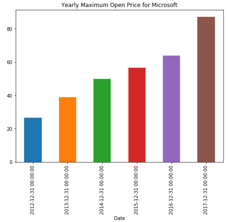
stock_data['Open'].resample('A').max().plot(kind='bar')
plt.title('Yearly Maximum Open Price for Microsoft')
The above script plots a bar plot showing the stock’s yearly maximum price. You can see that instead of the whole dataset, the resample method is only being applied to the Open column. The max() and plot() functions are chained together to 1) first find the maximum opening price for each year, and 2) plot the bar plot. The output looks like this:
Similarly, to plot the quarterly maximum opening price, we just set the offset value to ‘Q’:
plt.rcParams['figure.figsize'] = (8, 6) # change plot size
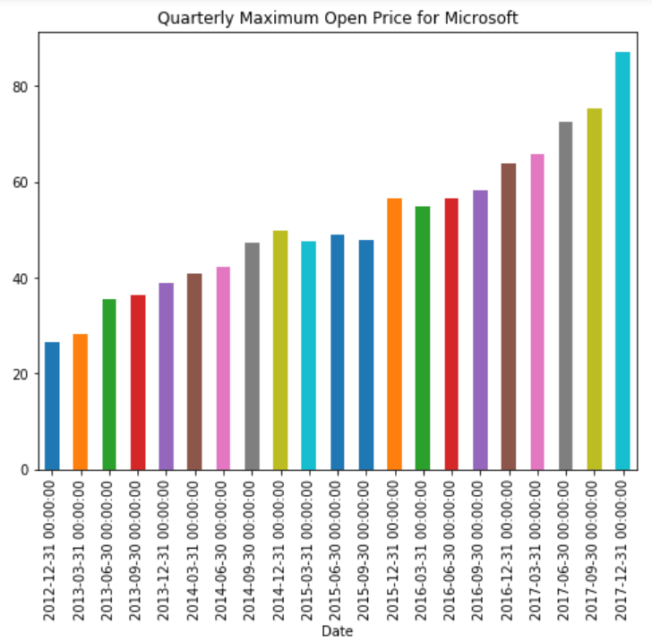
stock_data['Open'].resample('Q').max().plot(kind='bar')
plt.title('Quarterly Maximum Open Price for Microsoft')
Now you can see the quarterly maximum opening stock price for Microsoft:
Time Shifting
Time shifting refers to moving data forward or backward along the time index. Let’s see what we mean by shifting data forward or backward.
First, we’ll see what the first five rows and the last five rows of our dataset look like using the head() and tail() functions. The head() function displays the first five rows of the dataset, while the tail() function displays the last five rows.
Execute the following scripts:
stock_data.head()
stock_data.tail()
We printed the records from the head and tail of the dataset because when we later shift the data, we’ll see the differences between the actual and the shifted data.
Shifting Forward
Now let’s do the actual shifting. To shift the data forward, simply pass the number of indexes to move to the shift() method, as shown below:
stock_data.shift(1).head()
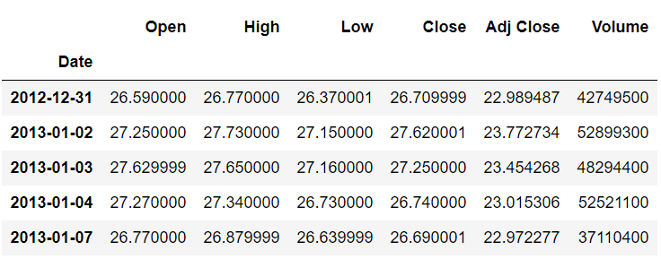
The above script moves our data one index forward, which means that the values for the Open, Close, Adjusted Close, and Volume columns that previously belonged to record N now belong to record N+1. The output looks like this:
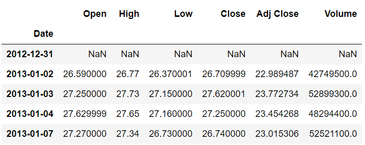
You can see from the output that the first index (2012-12-31) now has no data. The second index contains the records which previously belonged to the first index (2013-01-02).
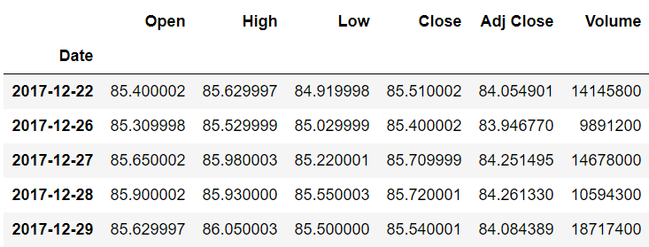
Similarly, at the tail, you will see that the last index (2017-12-29) now contains the records which previously belonged to the second-to-last index (2017-12-28). This is shown below:
Previously, the Open column value 85.900002 belonged to the index 2017-12-28, but after shifting one index forward, it now belongs to 2017-12-29.
Shifting Backwards
To shift the data backward, pass the number of indexes along with a minus sign. Shifting one index backward means that the values for the Open, Close, Adjusted Close, and Volume columns that previously belonged to record N now belong to record N-1.
To move one step backward, execute the following script:
stock_data.shift(-1).head()
The output looks like this:
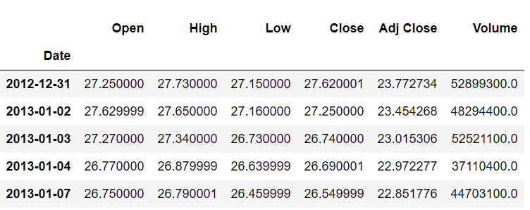
We can see that, after moving one index backward, the opening value of 27.250000 belongs to the index 2012-12-31. Previously, it belonged to the index 2013-01-02.
Shifting Data Using a Time Offset
In the time resampling section, we used an offset from the pandas offset table to specify the time period for resampling. We can use the same offset table for time shifting as well. To do so, we need to pass values for the periods and freq parameters of the tshift() function. The period attribute specifies the number of steps, while the freq attribute specifies the size of the step. For instance, if you want to shift your data two weeks forward, you can use the tshift() function as follows:
stock_data.tshift(periods=2,freq='W').head()
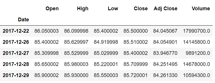
In the output, you will see data moved two weeks forward:
Learn More About Time Series Data in Python
Time series analysis is one of the major tasks that you will be required to do as a financial expert, along with portfolio analysis and short selling. In this article, you saw how Python’s pandas library can be used for visualizing time series data. You’ve learned how to perform time sampling and time shifting. However, this article barely scratches the surface of the use of pandas and Python for time series analysis. Python offers more advanced time series analysis capabilities, such as predicting future stock prices and performing rolling and expanding operations on time series data.
If you are interested in studying more about Python for time series analysis and other financial tasks, I highly recommend you enroll in our Python for data science introductory course to gain more hands-on experience.