Going Down to South Park, Part 3: TF-IDF Analysis with R

What Is TF-IDF Analysis?

Now let me introduce the method we'll be using: TF-IDF, which stands for term frequency-inverse document frequency. Wikipedia offers a nice explanation–it's a numerical statistic that's used to determine the importance of a given word to the context of a document that's part of a larger collection of documents.

Very common English words like the, a, and, etc. (known as stop words) are found in nearly every text. If we were to tally the words in a random document with just raw counts, these words would certainly be at the top.

To give you a better idea of how stop words can be misleading, let's look at the 10 most frequently occurring words in the entirety of South Park:

# Data frame with the 10 most frequent words in South Park
most_freq_words <- episode_words %>%
    count(word, sort = TRUE) %>%
    mutate(n = prettyNum(n, " ")) %>%
    head(10)

Word	Number of occurrences
you	28 277
the	27 690
to	22 228
i	20 167
a	17 326
and	15 201
it	11 218
is	10 768
of	10 658
we	10 230

See? We were right! There are no words with real meaning here that would tell us what the show is actually about. Rather, these words appear frequently simply because they're popular in the English language.

Here's another example to help make this more concrete: Imagine an author who's written several books, perhaps spanning multiple genres. Each book will contain certain words that are unique to its plot and context, but these words likely won't appear in the others. TF-IDF analysis will help us identify these unique words so we can get a better sense for what a document is about.

You'll see this later on in action with South Park–each episode contains unique lines of dialog with different words; TF-IDF will reveal the most important words for each episode. Because I know South Park very well, I'll personally evaluate the results of this analysis to see if it succeeded.

But How Does TF-IDF Work?

Okay, let's be more concrete. TF-IDF penalizes words that appear a lot and in a large number of documents. It's actually a combination of two different metrics, as the name suggests. The first metric is known as term frequency:

$$tf = \frac{number\ of\ term\ occurrences\ in\ a\ document}{total\ number\ of\ words\ in\ a\ document}$$

Simply put, term frequency is how often a given word is used in a document (as a percentage). We'll use the raw count of a word divided by the total number of words in a document to determine this metric. Easy enough, right?

The second part of TF-IDF is inverse document frequency:

$$idf = ln(\frac{n_{documents}}{n_{documents\ containing\ term}})$$

This statistic tells us if a word is rare or very common across a number of documents. For example, if we have 287 episodes of South Park and all 287 of them contain the word the, then our idf will be:

$$idf = ln(\frac{287}{287})=ln(1)=0$$

By multiplying these two metrics together, we get the TF-IDF:

$$tf\_idf = tf * idf$$

Note that the TF-IDF will always be 0 for words that appear in every document, since ln(1) is always 0.

Let's do a concrete example with the word alien. South Park episodes will be our documents; we'll calculate the term frequency for each episode in which the word 'alien' appears. Its inverse document frequency will be a single number. The following table captures all of these results for each episode where the word alien appears.

# Data frame of counts of "alien" word occurrences across episodes
alien <- filter(episode_words, word == "alien") %>%
    count(season_number, season_episode_number) %>%
    mutate(episode = glue("S{stringr::str_pad(season_number, 2, 'left', pad = '0')}E{stringr::str_pad(season_episode_number, 2, 'left', pad = '0')}")) %>%
    select(episode, n_alien = n) %>%
    left_join(
        by_episode %>% select(episode_number_str, total_words),
        by = c("episode" = "episode_number_str")) %>%
    # Calculating term frequency
    mutate(tf = n_alien / total_words)

# Wrangling alien to include idf and tf_idf columns
alien <- mutate(
    alien,
    # Calculating inverse document frequency
    idf = log(nrow(by_episode) / nrow(alien)),
    # Calculating term frequency-inverse document frequency
    tf_idf = tf * idf
)

episode	n_alien	total_words	tf	idf	tf_idf
S01E01	8	3234	0.0024737	2.886893	0.0071414
S01E11	1	3165	0.0003160	2.886893	0.0009121
S02E07	1	3100	0.0003226	2.886893	0.0009313
S03E03	4	3861	0.0010360	2.886893	0.0029908
S03E13	6	3005	0.0019967	2.886893	0.0057642
S05E05	1	3991	0.0002506	2.886893	0.0007234
S05E08	1	3390	0.0002950	2.886893	0.0008516
S05E12	1	3429	0.0002916	2.886893	0.0008419
S07E01	11	3225	0.0034109	2.886893	0.0098468
S07E12	1	3692	0.0002709	2.886893	0.0007819
S09E12	6	3339	0.0017969	2.886893	0.0051876
S11E11	1	2811	0.0003557	2.886893	0.0010270
S13E06	19	2859	0.0066457	2.886893	0.0191854
S14E01	14	3026	0.0046266	2.886893	0.0133564
S15E13	11	2947	0.0037326	2.886893	0.0107756
S20E01	1	3461	0.0002889	2.886893	0.0008341

Guessing the Topics of Seasons 18, 19, and 20

I'd like to dive into analyzing these three specific seasons, since each one has a cumulative plot that evolves throughout the episodes. This is something the creators have rarely done in the show-most other episodes stand alone and don't require too much knowledge of the previous ones.

This is perfect for us because we should be able to use TF-IDF to reveal what each season is about! You can imagine that this wouldn't be too meaningful for seasons where each episode has a different plot, right?

Let's examine the most significant words of these seasons in the following bar plot. The TF-IDF x-axis values are multiplied by 1000 so they're more readable.

# Start by counting word occurrences in each season
season_words <- episode_words %>%
    count(season_number, word, sort = TRUE)

# Calculate a total number of words for each season
total_words <- season_words %>%
    group_by(season_number) %>%
    summarize(total = sum(n))

# Join both of the data frames and calculate tf-idf for each word in the season
season_words <- left_join(season_words, total_words) %>%
    # Automatically calculate tf-idf using bind_tf_idf from tidytext
    bind_tf_idf(word, season_number, n) %>%
    arrange(desc(tf_idf))

# Filtered data frame with only top 10 tf-idf words from seasons 18, 19 and 20
our_season_words <- season_words %>%
    filter(season_number %in% c(18, 19, 20)) %>%
    group_by(season_number) %>%
    top_n(10, wt = tf_idf) %>%
    arrange(season_number, desc(tf_idf))

# This is a slightly modified our_season_words data frame which
# is needed in order to properly display the following bar plot.
top_n_season_words <- our_season_words %>%
    arrange(desc(n)) %>%
    group_by(season_number) %>%
    top_n(10) %>%
    ungroup() %>%
    arrange(season_number, tf_idf) %>%
    # This is needed for proper bar ordering in facets
    # https://drsimonj.svbtle.com/ordering-categories-within-ggplot2-facets
    mutate(order = row_number())

# Code to produce the following bar plot
ggplot(top_n_season_words, aes(order, tf_idf*1000, fill = factor(season_number))) +
    geom_col(show.legend = FALSE) +
    facet_wrap(~ season_number, scales = "free") +
    coord_flip() +
    labs(
        y = "tf-idf * 1000",
        x = "Top 10 most significant season topics"
    ) +
    scale_x_continuous(
        breaks = top_n_season_words$order,
        labels = top_n_season_words$word
    ) +
    scale_fill_manual(values = character_colors[c(2, 4, 6)]) +
    theme(panel.grid.minor = element_blank())

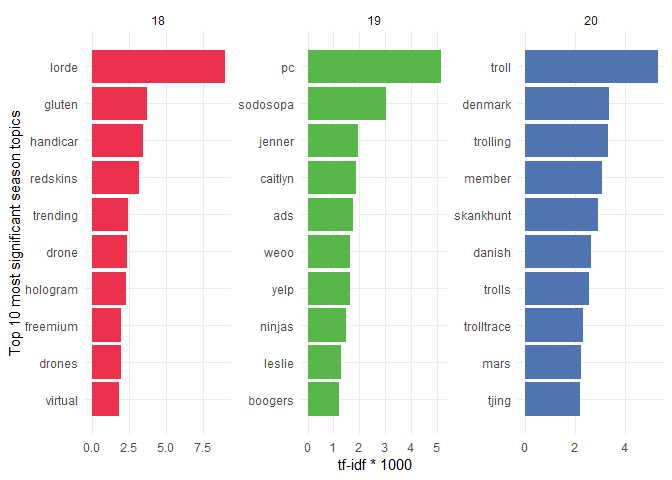
Let's now see how well the analysis turned out. The storyline of Season 18 focuses on Randy Marsh having a musical career as Lorde-and that happens to be the number-one word on our list! They also make fun of gluten-free diets throughout the season. A secondary but nonetheless big focus in this season is on virtual reality.

Season 19 has even stronger messages. It begins with an announcement that there will be a new principal: PC Principal. He starts promoting a PC (politically correct) culture because South Park is obviously full of racists and intolerant people. Mr. Garrison doesn’t take it anymore and starts running for President of the United States alongside his running mate Caitlyn Jenner—a former decathlon Olympic champion, Bruce Jenner, who had a sex change operation. The last important topic of the series is ads that negatively influence everything and even start being indistinguishable from regular people.

In Season 20, it was all about SkankHunt42, Kyle’s dad. He became a troll who enjoyed harassing all sorts of people online. It ended with the fictional Danish Olympic champion Freja Ollegard killing herself. Denmark then created a worldwide service called trolltrace.com that was able to identify any troll online. Eric Cartman also started dating Heidi Turner and tried to get to Mars with the help of Elon Musk’s SpaceX company.

If you compare the bold words with the ones in the bar plot, you’ll see that our TF–IDF analysis did a great job identifying the topics of these seasons! There were also a few words that were picked up that I didn’t mention (like drones or handicar); those were mainly significant in a few episodes, but they made it to the top 10 anyway. But overall, the method did great!

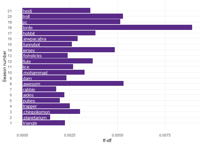
For the sake of completeness, the next bar plot shows you the most significant topic for each season. Just keep in mind that this doesn’t have to be true for the other seasons that we haven’t analyzed that closely, since not all seasons have a single theme:

# Summary data frame with each row being a top tf-idf word in a season
seasons_tf_idf <- season_words %>%
    group_by(season_number) %>%
    summarize(
        tf_idf = max(tf_idf),
        word = word[which.max(tf_idf)]
    )

# Code to produce the following plot
ggplot(seasons_tf_idf, aes(season_number, tf_idf, label = word)) +
    geom_col(fill = vertabelo_color) +
    geom_text(aes(y = 0), col = "white", hjust = -.05) +
    scale_x_continuous(breaks = 1:21) +
    labs(
        x = "Season number",
        y = "tf-idf"
    ) +
    coord_flip() +
    theme(panel.grid.minor = element_blank())

What Are the 3 Most Popular Episodes About?

I’ll do the same plot I did for the three seasons but now for the three most popular episodes (according to IMDB). Because episodes generally have a single, central theme, the results should be more accurate. Let’s find out!

# This code block is very similar to the one above that
# created the top 10 tf-idf words for the three seasons.
# Instead, it shows the top 10 tf-idf words for the 3 most
# popular South Park episodes.

ep_words <- episode_words %>%
    count(episode_order, word, sort = TRUE)

ep_total_words <- ep_words %>%
    group_by(episode_order) %>%
    summarize(total = sum(n))

ep_words <- left_join(ep_words, ep_total_words) %>%
     bind_tf_idf(word, episode_order, n) %>%
     arrange(desc(tf_idf))

eps_tf_idf <- ep_words %>%
    group_by(episode_order) %>%
    summarize(
        tf_idf = max(tf_idf),
        word = word[which.max(tf_idf)]
    )

top_episodes <- ep_words %>%
    group_by(episode_order) %>%
    top_n(10, wt = tf_idf) %>%
    arrange(episode_order, desc(tf_idf)) %>%
    filter(episode_order %in% c(69, 147, 92))

top_n_episode_words <- top_episodes %>%
    arrange(desc(n)) %>%
    group_by(episode_order) %>%
    top_n(10) %>%
    ungroup() %>%
    arrange(episode_order, tf_idf) %>%
    # This is needed for proper bar ordering in facets
    # https://drsimonj.svbtle.com/ordering-categories-within-ggplot2-facets
    mutate(order = row_number())

ggplot(top_n_episode_words, aes(order, tf_idf*100, fill = factor(episode_order, labels = c("Scott Tenorman Must Die", "The Return of the Fellowship of the Ring to the Two Towers", "Make Love, Not Warcraft")))) +
    geom_col(show.legend = FALSE) +
    facet_wrap(~ factor(episode_order, labels = c("Scott Tenorman Must Die", "The Return of the\n Fellowship of the Ring \nto the Two Towers", "Make Love, Not Warcraft")), scales = "free") +
    coord_flip() +
    labs(
        y = "tf-idf * 100",
        x = "Top 10 most significant episode topics"
    ) +
    scale_x_continuous(
        breaks = top_n_episode_words$order,
        labels = top_n_episode_words$word
    ) +
    scale_fill_manual(values = character_colors[c(2, 4, 6)]) +
    theme(panel.grid.minor = element_blank())

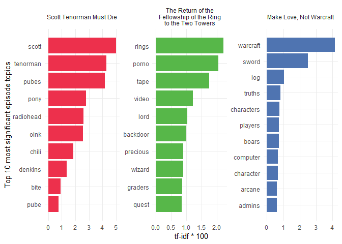
I’ll try to describe each of the three episodes using a few sentences with their true storyline.

Scott Tenorman Must Die: Scott Tenorman, a ninth grader, sells his pubes to Eric Cartman. Eric later realized that he got tricked and wants to get back at Scott, so he trains Mr. Denkins’s pony to bite off Scott’s wiener. Eric ends up having Scott’s parents killed and serves them to Scott in a chilli con carne at a chilli festival. The episode ends with Scott’s favorite band, Radiohead, coming to the festival and mocking Scott.
The Return of the Fellowship of the Ring to the Two Towers: Stan’s parents rent a porno video tape called Back Door Sl**s 9 and The Lord of the Rings. The boys are given a quest to deliver the LOTR movie to Butters. The two tapes get mixed up, though, and Butters is given the porno tape instead.
Make Love, Not Warcraft: The boys play World of Warcraft but encounter a player who’s even stronger than the admins and who starts killing innocent players. Their only way to level up to fight the bully character is to start killing computer-generated boars. Once they level their characters sufficiently, their only chance is to use the sword of a thousand truths to win the fight!

If you know these episodes, you must agree with these amazing results!

Let’s end this section with an overview of the main topics for each of the 287 episodes. You can explore the results in the following interactive plot. I put the IMDB ratings on the y-axis so that you can choose to only explore the popular episodes if you want:

# Wrangled by_episode data frame that includes the top tf-idf
# word for each episode.
by_episode <- inner_join(by_episode, eps_tf_idf) %>%
    mutate(text_hover = str_glue("Episode name: {episode_name}
                    Episode number: {episode_number_str}
                    IMDB rating: {rating}
                    Characteristic word: {word}"))
# Creating the following plot
g <- ggplot(by_episode, aes(episode_order, rating)) +
    geom_point(aes(text = text_hover), alpha = 0.6, size = 3, col = vertabelo_color) +
    labs(
        x = "Episode number",
        y = "IMDB rating"
    )
# Making the following plot interactive
ggplotly(g, tooltip = "text")

The End of the Series

Well, it’s been a real pleasure! This was the last article from the South Park text mining series, and I’ve had a lot of fun exploring this data with you! Let’s recap what we’ve learned to date:

I showed you where to get all the South Park dialog.
You learned how to create a dataset of words from spoken lines. This tidy data format helps you perform powerful data analysis more easily.
You used ggplot2 to create very informative plots, some of them even interactive thanks to the plotly package.
You even used a statistical proportion test to compare characters to see who is the naughtiest one, for example.

The last piece of knowledge you gained is how to identify document topics using TF–IDF analysis. It’s definitely a more sophisticated method than just using a raw count of words, which would inaccurately include stop words like “an” and “the.”

You also saw most of the code alongside the text. There are a few bits that I intentionally omitted. To see all of the code, visit my Github page as usual.

As always, reach out to me if you need any help with data analysis!

Patrik out.

Patrik Drhlik

Patrik is a freelance data scientist from Liberec, Czech Republic. He’s doing his PhD at the Technical University of Liberec, where he also teaches software engineering courses. He is highly passionate about the R programming language and data in general. He never leaves home without his Rubik’s cube and loves hitchhiking, athletics, mountains, kangaroos, and beer.

Going Down to South Park, Part 3: TF-IDF Analysis with R

What Is TF-IDF Analysis?

But How Does TF-IDF Work?

Guessing the Topics of Seasons 18, 19, and 20

What Are the 3 Most Popular Episodes About?

The End of the Series

Patrik Drhlik

18+ Best Online Resources for Learning SQL and Database Concepts (2020 revision)

Planning a Ski Trip with R Analysis

What Is TF-IDF Analysis?

But How Does TF-IDF Work?

Guessing the Topics of Seasons 18, 19, and 20

What Are the 3 Most Popular Episodes About?

The End of the Series

GET ACCESS TO EXPERT CONTENT

Patrik Drhlik

18+ Best Online Resources for Learning SQL and Database Concepts (2020 revision)

Planning a Ski Trip with R Analysis

Related Posts:

Going Down to South Park, Part 1: Text Analysis with R

Going Down to South Park, Part 2: Text Analysis with R

New Vertabelo Academy Course: Learn R with Introduction to R